Building a measure of change
Getting Started Measuring Change
Today I'm speaking to the Texas chapter of the Association of Change Management Professionals. The topic is "How to Define the Intangible and Justify the Return on Change Efforts."
For those who might find that presentation helpful, I wanted to show you how to use these techniques. This article will elaborate on how you can better develop your own measures of change.
I'd be remiss not to start by sharing the resources that were helpful to me in doing this. First is How to Measure Anything by Douglas Hubbard. I also found a lot of value in looking at the Signal and the Noise by Nate Silver and Decisive by Chip and Dan Heath.
I credit each of these books with starting me down this path and helping me evolve further as I learn more.
Step One: Determining What to Measure
In order for your measurements to be helpful, they have to be looking at the right details. The first step will be to find what you can estimate and measure to use as part of the formula that gives you results.
To measure the change, you must consider what part of that change is the significant variable. For example, to measure the impact of training I might look at the number of IT help-desk tickets. Does training result in fewer tickets? That might mean more productivity and less lost time.
To calculate this benefit, you might look at the number of people who use the system and the time they lose by not knowing how to do something. Provided, of course, they did not get training.
Your goal in this step is to think beyond the immediately clear metrics and focus on what matters. What is the benefit the change was supposed to realize? It wasn’t training as an end goal. It’s usually a business driver. Once you know that, you can find a variable that serves as a proxy for that business value (e.g. quality, time, money, etc.)
If you are measuring return on an enterprise system, you might look for time saved. To measure the benefit you could...
- Find the times the process happens per year...
- Then, multiply this by time the process takes...
- Finally, compare it to a probabilistic decrease in time spent after that point...
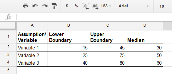
Consider all the variables that will factor into your formula and place them in your spreadsheet. I like to use an assumptions tab on its own. This way I can have the assumptions conversations without biasing my subject matter experts.
Step Two: Calibrating Your Estimates
This is where you (or your experts) will estimate the upper boundary, the lower boundary, and the median that drive the Monte Carlo simulation. Your goal is a 90% confidence interval on each of these values. This means is that 90% of the time the true value will lie above the lower threshold and below the upper threshold.
Take great care to try to push these two into as narrow range as possible without being overconfident. Hubbard explains if you ask people to pretend they're betting money on something they give a more accurate estimate. Look at each one by itself and ask questions to make sure they're approaching a more accurate number.
Ask someone if they would be willing to bet $100 to win $10 that the number is above their lowest threshold. Then ask them to make the same bet it would be below their upper threshold. Once you have those two numbers you can calculate the median.
The quality of your estimates will determine the quality of your simulations. Be sure to give them the attention they deserve.
Getting good estimates here is the most important part of the process. If your estimates are bad, your results won’t be helpful. But remember, people know more than they think. There is data and precedent out there to help you calibrate your ranges within reason. Find it and use it!
Step Three: Build Your Randomized Calculation
The driver for our Monte Carlo is using random ranges, with a normal distribution, based on our assumptions. Simulate that enough times, assess the results, and you should have a better (though not perfect) idea of what to expect. Remember, we are trying to reduce uncertainty and get a less ambiguous picture of what might happen. We cannot predict the future or get perfect results. But we can be more comfortable with our decisions.

Brute force with multivariate testing is a good way to reduce uncertainty.
For the building blocks of our multivariate Monte Carlo, we will use a formula to create a random number within the range. We will be following a normal distribution at a 90% confidence interval. Doing so will give you the inputs for the formula you will create in your regular simulations. An example of the formula is below:
=NORM.INV(RAND(), MEDIAN, (UPPERCELL-LOWERCELL)/3.29)
You might build a cell for each variable you will need randomized results for in your final simulation.
Hubbard outlines this method in his book, so full credit goes to him.
Step Four: Finish Your Spreadsheet
Once you have the variables you will be testing, you will need to build your formulas. This is where you take the results from each of the variables and pull them together to one simulated result.
An example might look like:
=Number of Times a Process Happens in a Year * Hours it normally Takes * Percentage Time Savings from Training
I tend to put the individual variables in their own cells, just so I can see the whole picture. You could pull them all in the same cell for the final if you want... but it might just result in a gnarly formula.
One you’ve got a row of simulations completed, you will want to copy that row down enough times to get a good sample size. Be sure to keep the variable cells (the ones pulling from your assumptions) as absolute references, and the final formula as relative (so they match the current row and don’t all refer back to one simulation). You can do this by using the "$" before the row and column identifiers for the cell (e.g. $A$1).
Step Five: Interpret Your Results
Now you have a series of rows giving you simulations. You will want to pull that data together so you can see the trend. I suggest building a bar graph using brackets of results. This will let you use the distribution of results in the simulation to tell you how likely a given result is.
What you get from this data will depend on what you are trying to learn. You can see how variable your upper and lower boundaries are. You can see how likely severe outliers are, which might tell you if you are facing a big risk.
You should also see the most likely distribution. This gives you some sense of what the outcome might be.
Conclusion
I put together a simple spreadsheet in Google Sheets that you can use as the foundation for your own model. Simply download a copy and build on it based on the steps outlined above.
I hope you find this helpful. If you’re interested in learning more, or you have any suggestions or questions, I’d love to hear them in the comments. Also, feel free to send me a message using the contact page.
Further Reading on Measuring Change and Decision Making:
I've developed my thinking on the measurement of change and decision-making with the help of several great books and resources. Here are some you might consider looking into:
- Douglas Hubbard – How to Measure Anything (Public Library | Amazon)
- Chip and Dan Heath – Decisive (Public Library | Amazon)
- Nate Silver – The Signal and The Noise (Public Library | Amazon)
- Daniel Kahneman – Thinking Fast and Slow (Public Library | Amazon)
- Gene Weingarten - The Washington Post - Pearls Before Breakfast